Using Sobol Sensitivity Analysis with an ODE

A sensitivity analysis example modeling forest growth.

Author

Affiliation

Published

May 22, 2023

Description

In this post, I perform a Sobol sensitivity analysis with an ODE (ordinary differential equation). This analysis is derived from an assignment for EDS230: Modeling Environmental Systems, as part of the curriculum for UCSB’s Master’s of Environmental Data Science program.

Sobol sensitivity analysis is a variance-based approach designed to efficiently sample a parameter space. Sobol quantifies sensitivity by breaking variance outputs into several indices, which are computed using parameter-output variance relationships. These indices include:

First Order Sensitivity (Main Effect): variance associated directly with parameter alone
Total Effect: variance associated with parameter and interaction with other parameters
Second Order Indices: quantification of how parameter pair-wise parameter interactions contribute to output variation

In this example, we consider the following model of forest growth (where forest size is measures in units of carbon (C)):

dC/dt = r ⋅ C for forests where C is below a threshold canopy closure

dC/dt = g ⋅ (1 - C/k) for forests where carbon is at or above the threshold canopy closure and K is a carrying capacity in units of carbon

The size of the forest (C), canopy closure threshold and carrying capacity are all in units of carbon. We think of the canopy closure threshold as the size of the forest at which growth rates change from exponential to linear, and we observe r, as early exponential growth rate and g as the linear growth rate once canopy closure is reached.

Implementing the Model

We begin the sensitivity analysis by implementing the model as a differential equation.

code

# carbon model

# c = forest size in measured in units of carbon
# ct = canopy threshold
# r = exponential growth rate
# g = linear growth rate at canopy closure
# k = carrying capacity

carbon_model <- function(Time, c, params) {
  
  ifelse(c < params$ct, 
          delta <- params$r * c,
          delta <- params$g * (1 - (c/params$k)))
  
  return(list(delta))
}

Running the Model with Set Parameters

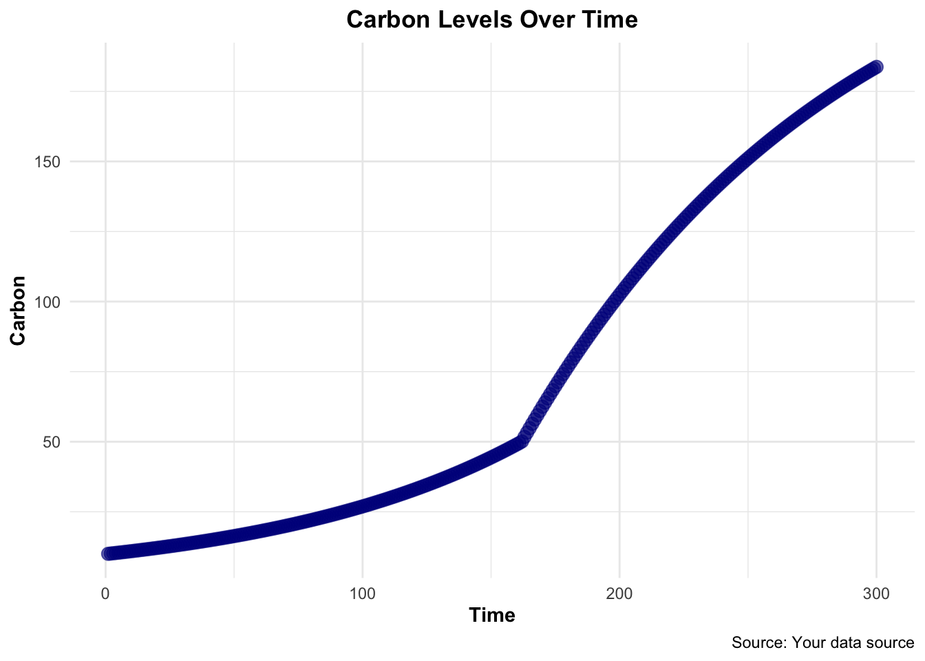
Once the model is implemented, we run the model for 300 years using given parameters, where there is no uncertainty. We begin with an initial forest size of 10 kg/C and the following parameters:

canopy closure threshold of 50 kgC
K = 250 kg C (carrying capacity)
r = 0.01 (exponential growth rate before canopy closure)
g = 2 kg/year (linear growth rate after canopy closure)

code

# initial forest size
c_init <- 10

# assignment of inital perameters
param <- list(
  ct = 50,
  k = 250,
  r = 0.01,
  g = 2
)

# 300 year simulation time
simtimes <- seq(from=1, to=300)

We utilize the ODE solver to run the model for 300 years

code

# ODE solver implementation
result <- ode(times = simtimes, 
              y = c(c = c_init), 
              func = carbon_model, 
              parms = param)

# column renaming
colnames(result) <- c("time","carbon")

# store results as a data frame
result <-  as.data.frame(result)

and then graph the trajectory results.

code

# graphing results 
ggplot(data = result, mapping = aes(x = time, y = carbon)) +
  geom_point(color = "darkblue", size = 3, alpha = 0.6) +
  labs(title = "Carbon Levels Over Time",
       x = "Time",
       y = "Carbon",
       caption = "Source: Your data source") +
  theme_minimal() +
  theme(plot.title = element_text(face = "bold", hjust = 0.5),
        axis.title = element_text(face = "bold"),
        plot.caption = element_text(hjust = 1))

Running a Sobol Global

After we have run the model with given parameters, we run a sobol global sensitivity analysis, varying all parameters at the same time. This will help us to explore how the estimated maximum forest size varies within the parameters:

pre-canopy closure growth rate (r)
post-canopy closure growth rate (g)
canopy closure threshold and carrying capacity (K)

For this exercise, we assume that parameters are all normally distributed with means as given in initial parameters and standard deviation of 10% of the mean value.

code

#set base params
ct_base = 50
k_base = 250
r_base = 0.01
g_base = 2

#set sd multiplier
sd = 0.1

#first set of parameter samples
ct <- rnorm(mean=ct_base, sd=ct_base*sd, n=300)
k <- rnorm(mean=k_base, sd=k_base*sd, n=300)
r <- rnorm(mean=r_base, sd=r_base*sd, n=300)
g <- rnorm(mean=g_base, sd=g_base*sd, n=300)
X1 = cbind.data.frame(ct=ct, k=k, r=r, g=g)

#repeat the process
ct <- rnorm(mean=ct_base, sd=ct_base*sd, n=300)
k <- rnorm(mean=k_base, sd=k_base*sd, n=300)
r <- rnorm(mean=r_base, sd=r_base*sd, n=300)
g <- rnorm(mean=g_base, sd=g_base*sd, n=300)
X2 = cbind.data.frame(ct=ct, k=k, r=r, g=g)

#mapping to account for negative values
X1 = X1 %>% map_df(pmax, 0.0)
X2 = X2 %>% map_df(pmax, 0.0)

#sobol parameters
sens_carbon <- sobolSalt(model = NULL, X1, X2, nboot = 300)

# naming output columns 
colnames(sens_carbon$X) <- c("ct","k", "r", "g")

code

# function to return max carbon  
compute_max = function(results) {
  
  max_carbon = results$carbon[300]
  
  return(list(max_carbon = max_carbon))
}

# function for ODEsolve
carbon_wrapper <- function(c_initial, ct, k, r, g, simtimes, func) {
  parms = list(ct=ct, k=k, r=r, g=g)
  results = ode(y= c_initial, times= simtimes, func= func, parms= parms)
  colnames(results) = c("time","carbon")
  metrics = compute_max(as.data.frame(results))
  return(metrics)
}

code

allresults = as.data.frame(sens_carbon$X) %>% 
  pmap(carbon_wrapper, 
       c_initial=c_init, 
       simtimes=simtimes, 
       func=carbon_model)

#take the results out of the list 
allres = allresults %>% map_dfr(`[`,c("max_carbon"))

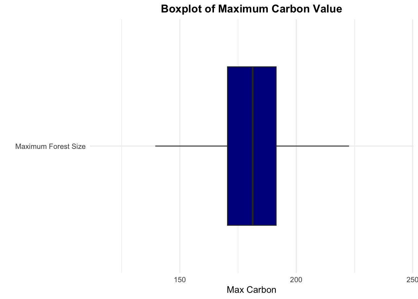
We graph the results of the sensitivity analysis as a boxplot of maximum forest size and record sobol indices S and T.

code

# box plot of max carbon
ggplot(data = allres, aes(x = "Maximum Forest Size", y = max_carbon)) +
  geom_boxplot(fill = "darkblue", outlier.shape = NA) +
  labs(title = "Boxplot of Maximum Carbon Value",
       y = "Max Carbon",
       x = "") +
  theme_minimal() +
  theme(plot.title = element_text(face = "bold", hjust = 0.5),
        axis.title.y = element_text(face = "bold"),
        plot.caption = element_text(hjust = 1)) +
  coord_flip()

code

# record the indices
sens_carbon_maxcarbon = sensitivity::tell(sens_carbon,allres$max_carbon)

# First-order indices table
first_order_indices <- sens_carbon_maxcarbon$S
rownames(first_order_indices) <- c("ct", "k", "r", "g")  # Rename rows with variable names
kable_first_order <- kable(first_order_indices, caption = "First-Order Indices") %>%
  kable_styling("striped", full_width = FALSE) 

# Total sensitivity index table
total_sensitivity_index <- sens_carbon_maxcarbon$T
rownames(total_sensitivity_index) <- c("ct", "k", "r", "g")  # Rename rows with variable names
kable_total_sensitivity <- kable(total_sensitivity_index, caption = "Total Sensitivity Index") %>%
  kable_styling("striped", full_width = FALSE)

# Print the tables
kable_first_order

First-Order Indices
	original	bias	std. error	min. c.i.	max. c.i.
ct	0.0535712	0.0041386	0.0589892	-0.0559964	0.1613757
k	0.3609487	0.0015147	0.0547030	0.2594734	0.4711013
r	0.3166746	0.0019369	0.0588323	0.1962994	0.4350840
g	0.2003974	0.0028063	0.0532262	0.0877141	0.3037629

code

kable_total_sensitivity

Total Sensitivity Index
	original	bias	std. error	min. c.i.	max. c.i.
ct	0.0559747	0.0005506	0.0060035	0.0428226	0.0667686
k	0.3502126	0.0002552	0.0352006	0.2790502	0.4169600
r	0.3385371	0.0041040	0.0363116	0.2525754	0.3986892
g	0.2256922	0.0015620	0.0240854	0.1751392	0.2664142

Considering the range of parameter variations, a shift exceeding 50% in the maximum carbon levels within the forest becomes apparent. Notably, both the first-order and total sensitivity analyses underscore the significance of the carrying capacity (k) and exponential growth rate (r) as pivotal factors in influencing the extent of variability in maximum carbon levels. Foreseeing the potential impact of climate change on forest dynamics, it is plausible to anticipate alterations in the carrying capacity. For instance, factors such as soil nutrient depletion could curtail the forest’s capacity to support tree growth. In light of this scenario, a corresponding decline in the overall carbon content within forests could be anticipated.

--- title: "Using Sobol Sensitivity Analysis with an ODE" description: "A sensitivity analysis example modeling forest growth." author: - name: Gabrielle Smith url: https://gabriellensmith.github.io affiliation: MEDS affiliation-url: https://ucsb-meds.github.io/ date: 2023-05-22 catergories: [MEDS, Modeling, R] image: forest.jpeg editor: visual toc: true draft: false format: html: code-fold: true code-tools: true code-summary: 'code' --- ## Description In this post, I perform a Sobol sensitivity analysis with an ODE (ordinary differential equation). This analysis is derived from an assignment for EDS230: Modeling Environmental Systems, as part of the curriculum for UCSB's Master's of Environmental Data Science program. Sobol sensitivity analysis is a variance-based approach designed to efficiently sample a parameter space. Sobol quantifies sensitivity by breaking variance outputs into several indices, which are computed using parameter-output variance relationships. These indices include: - First Order Sensitivity (Main Effect): variance associated directly with parameter alone - Total Effect: variance associated with parameter and interaction with other parameters - Second Order Indices: quantification of how parameter pair-wise parameter interactions contribute to output variation In this example, we consider the following model of forest growth (where forest size is measures in units of carbon (C)): *dC/dt = r ⋅ C* for forests where C is below a threshold canopy closure *dC/dt = g ⋅ (1 - C/k)* for forests where carbon is at or above the threshold canopy closure and K is a carrying capacity in units of carbon The size of the forest *(C)*, canopy closure threshold and carrying capacity are all in units of carbon. We think of the canopy closure threshold as the size of the forest at which growth rates change from exponential to linear, and we observe *r*, as early exponential growth rate and *g* as the linear growth rate once canopy closure is reached. ## Implementing the Model We begin the sensitivity analysis by implementing the model as a differential equation. ```{r include=FALSE} # packages rm(list = ls()) if ("package:kableExtra" %in% search()) { detach("package:kableExtra", unload=TRUE) } library(tidyverse) library(deSolve) library(sensitivity) library(knitr) library(kableExtra) library(sjPlot) ``` ```{r} # carbon model # c = forest size in measured in units of carbon # ct = canopy threshold # r = exponential growth rate # g = linear growth rate at canopy closure # k = carrying capacity carbon_model <- function(Time, c, params) { ifelse(c < params$ct, delta <- params$r * c, delta <- params$g * (1 - (c/params$k))) return(list(delta)) } ``` ## Running the Model with Set Parameters Once the model is implemented, we run the model for 300 years using given parameters, where there is no uncertainty. We begin with an initial forest size of 10 kg/C and the following parameters: - canopy closure threshold of 50 kgC - *K* = 250 kg C (carrying capacity) - *r* = 0.01 (exponential growth rate before canopy closure) - *g* = 2 kg/year (linear growth rate after canopy closure) ```{r} # initial forest size c_init <- 10 # assignment of inital perameters param <- list( ct = 50, k = 250, r = 0.01, g = 2 ) # 300 year simulation time simtimes <- seq(from=1, to=300) ``` We utilize the ODE solver to run the model for 300 years ```{r} # ODE solver implementation result <- ode(times = simtimes, y = c(c = c_init), func = carbon_model, parms = param) # column renaming colnames(result) <- c("time","carbon") # store results as a data frame result <- as.data.frame(result) ``` and then graph the trajectory results. ```{r} # graphing results ggplot(data = result, mapping = aes(x = time, y = carbon)) + geom_point(color = "darkblue", size = 3, alpha = 0.6) + labs(title = "Carbon Levels Over Time", x = "Time", y = "Carbon", caption = "Source: Your data source") + theme_minimal() + theme(plot.title = element_text(face = "bold", hjust = 0.5), axis.title = element_text(face = "bold"), plot.caption = element_text(hjust = 1)) ``` ## Running a Sobol Global After we have run the model with given parameters, we run a sobol global sensitivity analysis, varying all parameters at the same time. This will help us to explore how the estimated **maximum forest size** varies within the parameters: - pre-canopy closure growth rate (*r*) - post-canopy closure growth rate (*g*) - canopy closure threshold and carrying capacity (*K*) For this exercise, we assume that parameters are all normally distributed with means as given in initial parameters and standard deviation of 10% of the mean value. ```{r} #set base params ct_base = 50 k_base = 250 r_base = 0.01 g_base = 2 #set sd multiplier sd = 0.1 #first set of parameter samples ct <- rnorm(mean=ct_base, sd=ct_base*sd, n=300) k <- rnorm(mean=k_base, sd=k_base*sd, n=300) r <- rnorm(mean=r_base, sd=r_base*sd, n=300) g <- rnorm(mean=g_base, sd=g_base*sd, n=300) X1 = cbind.data.frame(ct=ct, k=k, r=r, g=g) #repeat the process ct <- rnorm(mean=ct_base, sd=ct_base*sd, n=300) k <- rnorm(mean=k_base, sd=k_base*sd, n=300) r <- rnorm(mean=r_base, sd=r_base*sd, n=300) g <- rnorm(mean=g_base, sd=g_base*sd, n=300) X2 = cbind.data.frame(ct=ct, k=k, r=r, g=g) #mapping to account for negative values X1 = X1 %>% map_df(pmax, 0.0) X2 = X2 %>% map_df(pmax, 0.0) #sobol parameters sens_carbon <- sobolSalt(model = NULL, X1, X2, nboot = 300) # naming output columns colnames(sens_carbon$X) <- c("ct","k", "r", "g") ``` ```{r} # function to return max carbon compute_max = function(results) { max_carbon = results$carbon[300] return(list(max_carbon = max_carbon)) } # function for ODEsolve carbon_wrapper <- function(c_initial, ct, k, r, g, simtimes, func) { parms = list(ct=ct, k=k, r=r, g=g) results = ode(y= c_initial, times= simtimes, func= func, parms= parms) colnames(results) = c("time","carbon") metrics = compute_max(as.data.frame(results)) return(metrics) } ``` ```{r} allresults = as.data.frame(sens_carbon$X) %>% pmap(carbon_wrapper, c_initial=c_init, simtimes=simtimes, func=carbon_model) #take the results out of the list allres = allresults %>% map_dfr(`[`,c("max_carbon")) ``` We graph the results of the sensitivity analysis as a boxplot of maximum forest size and record sobol indices **S** and **T**. ```{r} # box plot of max carbon ggplot(data = allres, aes(x = "Maximum Forest Size", y = max_carbon)) + geom_boxplot(fill = "darkblue", outlier.shape = NA) + labs(title = "Boxplot of Maximum Carbon Value", y = "Max Carbon", x = "") + theme_minimal() + theme(plot.title = element_text(face = "bold", hjust = 0.5), axis.title.y = element_text(face = "bold"), plot.caption = element_text(hjust = 1)) + coord_flip() ``` ```{r} # record the indices sens_carbon_maxcarbon = sensitivity::tell(sens_carbon,allres$max_carbon) # First-order indices table first_order_indices <- sens_carbon_maxcarbon$S rownames(first_order_indices) <- c("ct", "k", "r", "g") # Rename rows with variable names kable_first_order <- kable(first_order_indices, caption = "First-Order Indices") %>% kable_styling("striped", full_width = FALSE) # Total sensitivity index table total_sensitivity_index <- sens_carbon_maxcarbon$T rownames(total_sensitivity_index) <- c("ct", "k", "r", "g") # Rename rows with variable names kable_total_sensitivity <- kable(total_sensitivity_index, caption = "Total Sensitivity Index") %>% kable_styling("striped", full_width = FALSE) # Print the tables kable_first_order kable_total_sensitivity ``` Considering the range of parameter variations, a shift exceeding 50% in the maximum carbon levels within the forest becomes apparent. Notably, both the first-order and total sensitivity analyses underscore the significance of the carrying capacity (k) and exponential growth rate (r) as pivotal factors in influencing the extent of variability in maximum carbon levels. Foreseeing the potential impact of climate change on forest dynamics, it is plausible to anticipate alterations in the carrying capacity. For instance, factors such as soil nutrient depletion could curtail the forest's capacity to support tree growth. In light of this scenario, a corresponding decline in the overall carbon content within forests could be anticipated.